Neural networks
Construction of a neural network (NN) interatomic potential requires three steps:
generation of reference data, i.e., ab initio energy and, optionally, forces for relevant structures
data parsing, i.e., converting the structural data into suitable NN input
model training, i.e., fitting the NN model’s parameters to the reference data
The following sections overview these steps in the framework of the MAISE package.
Reference data generation
An ab initio dataset can be generated with any code that produces
standard target values for training NN models with MAISE: total
energies and atomic forces. Although the ab initio method for
reference calculations is chosen by the user, the data should be
represented in a particular way to be readable by MAISE. The
structural information should be specified in the VASP POSCAR file
format and named POSCAR.0 while the total energy, unit cell stress
components (currently not used for NN training), and atomic forces
corresponding to each structure should be given in a dat.dat file
with the following format:
    -18.53179845
  in kB      98.74889    86.74652   101.67959    -6.14884     0.63009    -0.13363
 POSITION                                       TOTAL-FORCE (eV/Angst)
 -----------------------------------------------------------------------------------
      5.76733      2.45539      0.22001         0.008141      0.036506     -0.024264
      2.01046      0.80759      0.20241        -0.008141     -0.036484      0.024354
      3.04507      3.37524     -0.02824         0.020516      0.042442     -0.010660
      3.12997      0.73792      2.92859        -0.000007     -0.000032      0.000257
      6.84094      2.41756      2.80406        -0.020509     -0.042431      0.010312
 -----------------------------------------------------------------------------------
    total drift:                               -0.000016      0.000196     -0.000228
This information can be easily extracted from an OUTCAR file of a single-point total energy/enthalpy VASP calculation using these bash commands:
grep y= OUTCAR |awk '{print $7}'              > dat.dat
grep 'in kB' OUTCAR                          >> dat.dat
grep -A 10000 POSI  OUTCAR |sed '/drift/q'   >> dat.dat
Each data directory should contain only one pair of the corresponding
POSCAR.0 and dat.dat files. The full set of directories should
be organized in a particular fashion for MAISE to proprely process the
data into training and testing sets. The following diagram illustrates
the exected hierarchy, while the Data parsing section provides
further details on data organization.
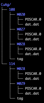
In this structure, each data point (a pair of POSCAR.0 and
dat.dat files) should be inside a directory and the collection of
these data points should be in a parent directory, e.g.,
main_dir/.
In this example, MAISE will process the full directory CuAg
specified in the setup file with the DEPO FLAG. It will
determine that the are two direct subdirectories, or batches, and
treat each batch as a group of comparable data in terms of
composition, dimensionality, conditions, etc. For instance, 108
could be a collection of 3D crystal structures evaluated at 0 GPa,
while 114 could be a set of small clusters. This separation allows
MAISE to filter out unphysical or irrelevant structures using settings
in the setup file. By optionally placing a tag file in a
subdirectory, one can overwrite the settings for that
batch. Please see Data filtering options for more detail.
Note
In Ref. [1] we introduced our approach to generate the NN training data using unconstrained evolutionary searches. Further generatlizaion of that approach is provided in our recent study [2] in which dataset generation is carried out in cycles of evolutionary runs. As discussed in these studies, we have found the following list to be good practices in dataset generation:
inclusion of some customized data to the training set, e.g., equation of state (EOS) data for select structures (the dimer, FCC, BCC, HCP, etc.) as they teach the NN to disfavor unphysical configurations that can be inadvertently probed in global searches or MD runs
elimination of structures that are either too similar to each other or clearly irrelevant to the regions of configuration space that are not of our interest for the problem in hand
exclusion of structures with unphysically high energy or forces
Data parsing
The data processing step allows the user to filter out irrelevant
configurations, earmark structures for training and testing, and parse
atomic environments into NN inputs. Here, the idea is to precompute
and store NN inputs for each structure only once to avoid performing
this costly operation at each NN fitting step. Data parsing is done in
a single run with JOBT = 30 FLAG in the setup file,
produces a file for each structure with parsed energy/force NN
inputs, and collects statistics on the energy, force, volume, and RDF
distributions in the full dataset. Parsing task includes filtering,
earmarking, and parsing operations. These operations can be customized
by (i) choosing FLAGs in the setup file; (ii) arranging the data
by type into subdirectories and specifying energy thresholds and
intended application type (training or testing) for acceptable data in
tag file; (iii) and specifying Behler-Parrinello (BP) symmetry
functions [3] in the basis file for converting atomic
environments into NN input.
Data parsing setup
Table 1 lists FLAGs in the MAISE setup file that define
the data parsing task.
FLAG |
Short description |
|---|---|
Data parsing (30) |
|
Number of the cores for parsing task |
|
Parsing for: Energy (0); Energy-Force (1) |
|
Fraction of atoms that will be parsed to use for EF training |
|
Number of element types for dataset parsing and training |
|
Atomic number of the elements specified with NSPC tag |
|
The length of the input vector of the neural network |
|
Parse only this fraction of lowest-energy structures (from 0 to 1) |
|
Maximum energy from the lowest-energy structure that is parsed |
|
Will not parse data with forces larger than this value |
|
Random seed for the parsing: time (0); seed value (+); no randomization (-) |
|
Path to the DFT datasets to be parsed |
|
Location of the parsed data to write the parsed data |
JOBT , set to 30, initiates the parsing task.
NPAR is number of cores to be used in the parsing job. The parallelization is done with over atoms in each structure.
TEFS defines what type of data parsing is performed for subsequent use in the NN model training and testing. In TEFS = 0 parsing, only energy (E) data is processed. In TEFS = 1 parsing, both energy and force (EF) data are processed.
FMRK is a real number between 0.0 and 1.0 defining what fraction of atoms in each structure, provided that TEFS = 1, will be processed for subsequent energy-force training. For each marked atom, the code parses all x, y, and z components of the force. Note that forces below \(10^{-5}\) eV/A are ignored, as they are likely close to zero by symmetry.
NSPC is the total number of the atomic species that are present in the dataset.
TSPC is a list of all species atomic numbers present in the dataset. This list should be ordered from the lowest to highest atomic number.
NSYM is the total number of the BP symmetry functions that will be used
for data parsing. This number should match the number of the
introduced symmetry functions in the basis file.
NCMP is the total number of the input vector component (per species in case of the multi-component systems) which will be produced from the introduced BP symmetry functions. This number depends on the number of species in the system (NSPC) and the number of the radial and angular functions in that total. Having N2 and N3 radial and angular BP functions, this number will be equal to
NSPC \(\times\)N2+ NSPC \(\times\)(NSPC-1)\(\times\)…\(\times\)1\(\times\)N3.
If the user does not provide the correct input number for NCMP, MAISE will exit with a message that suggests the correct number.
ECUT is a a real number between 0.0 and 1.0 defining what fraction of the lowest-enthalpy structures will be kept in each batch (see Reference data generation) after the structures in the batch are ranked by enthalpy per atom. The default value is 0.9
EMAX is a cutoff in eV/atom for the highest energy structure that will be parsed. This energy window is measured with respect to the lowest enthalpy structure in each batch. The default value is 5.0 eV/atom.
FMAX is a cutoff in eV/A. Any structure with an atomic force component higher than this value will not be parsed. The default value is 50 eV/A.
RAND is a random number seed that determines the arrangement of the structures in the training and testing sets. for RAND = 0 system time will be used, a RAND > 0 value will be used as seed, and for any RAND < 0 the structures will be parsed in the order they appear in the operating system list output. This list of parsed structures will be used at the training stage to pick training and testing sets.
DEPO is a path to the DFT data to be parsed. MAISE expects the dataset to be arranged in a format described in the Reference data generation section.
DATA is a path to the location in which the parsed data will be stored.
Data filtering options
In data filtering, the ECUT, EMAX, and FMAX FLAGs described in the table of setup parameters control the maximum values of energy (enthalpy) and
forces allowed in the database. A single energy cutoff is ill-defined
or not helpful if the database contains entries with different
structure types (clusters or crystal structures), compositions (in
multielement systems), or simulation conditions (pressure
values). Provided that the data is sorted into batch subdirectories
by type, ECUT and EMAX are applied to the
energy per atom within each subset. These values can be overwritten
for a specific subset by placing a tag file in the corresponding
subdirectory. This tag file can also be used to promote the
inclusion of the subset, e.g., EOS data, into the training set.
This is an example of a tag file illustrating which setup FLAGs
will be overwritten when this batch subdirectory is prossessed.
1              # (1) train+test (2) train only # (3) test only  (4) discard folder
0.9            # ECUT
2.0            # EMAX
5.0            # FMAX
Behler-Parrinello descriptor
MAISE relies on BP symmetry functions for describing the atomic
environments [9][10]. A customizable set of BP functions is defined
in the basis file. Below is an example of a basis with a
typical descriptor that has been used for generating the standard
library of NN models in MAISE. In this set of models, we typically use
51 functions per element with the cutoff expanded from 6.0 A to 7.5 A
and the corresponding η parameters rescaled by a factor of
1/(1.25*1.25) (for more details see our previous study [4]).
The GN values of (2 and 4) correspond to the pair and triplet BP functions defined as (G1 and G2) in Ref. [9] or as (G2 and G4) in Ref. [10]. n1 and n2 are eta parameters in the G2 and G4 functions while l is lambda in G4. k is an obsolete parameter no longer used in the BP functions. z is the zeta power value in G4.
The original set of BP parameters was defined in Bohrs while MAISE performs calculations in Angstroms. So, if the Rc, n1, and n2 parameters are specified in Bohrs, they will be converted to Angstroms using this a = 0.529177249 conversion factor as follows: Rc = a*Rc, n1 = n1/(a*a), and n2 = n2/(a*a). The original BP functions cutoff radius was 6.0 Ang, while our current default is 7.5 Ang. So, we use r = 1.25 to rescale these parameters in the same way: Rc = r*Rc, n1 = n1/(r*r), and n2 = n2/(r*r). Note that if you define your own BP parameters in Angstroms, you can set both a and r to 1.0.
  B2A          Scaling
  0.529177249  1.25

  N  GN  Rc  Rs   n1  n2  k   z   l

  1   2   0   0   0   0   0   0   0
  2   2   0   0   1   0   0   0   0
  3   2   0   0   2   0   0   0   0
  4   2   0   0   3   0   0   0   0
  5   2   0   0   4   0   0   0   0
  6   2   0   0   5   0   0   0   0
  7   2   0   0   6   0   0   0   0
  8   2   0   0   7   0   0   0   0
  9   4   0   0   0   0   0   0   0
 10   4   0   0   0   0   0   0   1
 11   4   0   0   0   0   0   1   0
 12   4   0   0   0   0   0   1   1
 13   4   0   0   0   1   0   0   0
 14   4   0   0   0   1   0   0   1
 15   4   0   0   0   1   0   1   0
 16   4   0   0   0   1   0   1   1
 17   4   0   0   0   2   0   0   0
 18   4   0   0   0   2   0   0   1
 19   4   0   0   0   2   0   1   0
 20   4   0   0   0   2   0   1   1
 21   4   0   0   0   3   0   0   0
 22   4   0   0   0   3   0   0   1
 23   4   0   0   0   3   0   1   0
 24   4   0   0   0   3   0   1   1
 25   4   0   0   0   3   0   2   0
 26   4   0   0   0   3   0   2   1
 27   4   0   0   0   3   0   3   0
 28   4   0   0   0   3   0   3   1
 29   4   0   0   0   4   0   0   0
 30   4   0   0   0   4   0   0   1
 31   4   0   0   0   4   0   1   0
 32   4   0   0   0   4   0   1   1
 33   4   0   0   0   4   0   2   0
 34   4   0   0   0   4   0   2   1
 35   4   0   0   0   4   0   3   0
 36   4   0   0   0   4   0   3   1
 37   4   0   0   0   5   0   0   0
 38   4   0   0   0   5   0   0   1
 39   4   0   0   0   5   0   1   0
 40   4   0   0   0   5   0   1   1
 41   4   0   0   0   5   0   2   0
 42   4   0   0   0   5   0   2   1
 43   4   0   0   0   5   0   3   0
 44   4   0   0   0   5   0   3   1
 45   4   0   0   0   6   0   0   0
 46   4   0   0   0   6   0   0   1
 47   4   0   0   0   6   0   1   0
 48   4   0   0   0   6   0   1   1
 49   4   0   0   0   6   0   2   0
 50   4   0   0   0   6   0   2   1
 51   4   0   0   0   6   0   3   0

 Rc   1   11.338
 Rs   1   0.0000
 n1   8   0.0010   0.0100   0.0200   0.0350   0.0600   0.1000   0.2000   0.4000
 n2   7   0.0001   0.0030   0.0080   0.0150   0.0250   0.0450   0.0800
 k    1   1.0000
 z    4   1.0000   2.0000   4.0000  16.0000
 l    2  -1.0000   1.0000
Data parsing execution
With the required input files, i.e., setup and basis files in the
current directory, the parsing task can be performed by running MAISE:
$ maise
For a typical database of a few thousand medium-size structures, the job takes a few minutes.
Data parsing output
The output of the data parsing job is as follows:
A set of
e*files contains the ab initio target energy/force values along with structural information converted to NN input vectors with the helpf of the chosen the BP symmetry functions. Thesee*files will be imported at the time of NN fitting to create the training and testing sets.A
stamp.datfile summarizes the most important parameters/specifications of the parsed data. An example of thestamp.datfile is presented here:
VERS   maise.2.6.00
TIME   Sat Jul 14 01:54:05 2020
DEPO   /mnt/Storage/home/samad/GEN/AuSn/DAT/
STRC   3991
PRSE   3358
PEFS   1
FMRK   0.500000
PRSF   28770
COMP   145
NSYM   51
NSPC   2
TSPC   79 50
NMAX   20
RAND   5
ECUT   0.900000
EMAX   5.000000
FMAX   50.000000
index.datfile contains an ordered list of the parsed structures. The order is determined by the RAND FLAG in the parsing setup.ve.datcontains a list of the volume per atom, energy per atom, and maximum atomic force component for each parsed structure.RDFP.datfile is the average RDF profile of the parsed dataset.
Neural network training
The default NN implemented in MAISE has a standard feed-forward architecture with one bias per input or hidden layer. Signals are processed with hyperbolic activation functions in hidden layers and with the linear function in the output neuron.
The filtered and parsed data can be split into training and testing
sets; data earmarked for training with tag files in the
corresponding subdirectories (see Data filtering options section)
has a higher priority to be placed into the training set.
NN fitting via backpropagation can be performed with BFGS [5] or CG [6] algorithm as implemented in the GSL [7] by minimizing the root-mean-square-error between target and NN output values. Energy-only (E) and energy-force (EF) training types are available. For the latter, please make sure that the data is parsed into both energy and force NN inputs (FLAG TEFS =1).
Besides the traditional full training in which all NN weights are optimized, MAISE has an option to use the stratified and generalized stratified training schemes. These approaches are briefly introduced in the following sections, while a detailed description of these schemes is available in Refs. [1] and [2], respectively.
NN training setup
A NN training job is fully configured in a single setup file.
FLAG |
Short description |
|---|---|
Training type: full training (40); stratified training (41) |
|
Number of cores for parallel training |
|
The optimizer algorithm for neural network training |
|
Number of the optimization steps for training |
|
Error tolerance for training |
|
Training target value: E (0); EF (1) |
|
Number of element types for dataset parsing and training |
|
Atomic number of the elements specified with NSPC tag |
|
Mumber of the BP symmetry functions for parsing data |
|
The length of the input vector of the neural network |
|
Number of structures used for training (negative number means percentage) |
|
Number of structures used for testing (negative number means percentage) |
|
Number of hidden layers (does not include input vector and output neuron) |
|
Number of neurons in hidden layers |
|
Activation function of the hidden layers’ neurons: linear (0); tanh (1) |
|
Regularization parameter |
|
Rand seed for generating NN weights (0 for system time) |
|
Location of the parsed data to read from for training |
|
Directory for storing model parameters in the training process |
|
Directory for model testing data |
JOBT specifies the training task and its type:
40 full training
41 stratified training
NPAR is the number of the cores to be used for the NN training. Here, the parallelization is done over all structures in the training/testing set.
MINT specified the type of the optimizer to be used for the NN training. BFGS2 typically provides the most efficient optimization.
0 BFGS2
1 CG-FR
2 CG-PR
3 steepest descent
MITR is the number of the optimization steps (epochs) to be performed in the NN training task.
ETOL is a minimization stopping criterion. The training exits if the difference between the total errors for two subsequent steps falls below this value. Usually, it is better to set ETOL to a very small value and control the length of NN training with the MITR FLAG.
TEFS is type of the target value to be used in the NN training:
0 energy only
1 energy and force
This FLAG should be consistent with the corresponding TEFS. FLAG in the data parsing. Force training is possible only if the force data is processed during the parsing stage.
NSPC is the total number of the atomic species that are present in the dataset.
TSPC is a list of all species atomic numbers present in the dataset. This list should be ordered from the lowest to highest atomic number.
NSYM is the total number of the BP symmetry functions used for
data parsing. This number should match the number of the introduced
symmetry functions in the basis file. It should be consistent with
the the corresponding value used at the parsing stage. The value can be
retrieved from the stamp.dat file.
NCMP is the total number of the input vector component (per species in
case of the multi-component systems) which will be produced from the
introduced BP symmetry functions. It should be consistent with
the the corresponding value used at the parsing stage. The value can be
retrieved from the stamp.dat file.
NTRN is the number (if NTRN is positive) or the fraction (if
NTRN is negative) of the parsed data which will be used for the NN
training. At the time of the parsing, a list of structures is
generated in the index.dat file in the parsed data location; the
NTRN FLAG will read that list and import NTRN number/percent
of the data from the beginning of the list for training.
NTST is the number (if NTST is positive) or the fraction (if
NTST is negative) of the parsed data which will be used for the NN
testing. At the time of the parsing, a list of structures is
generated in the index.dat file in the parsed data location; the
NTST FLAG will read that list and import NTST number/percent
of the data from the end of the list for the NN testing.
NNNN is the number of the hiddern layers in the NN excluding the input and the single-neuron output layers. Currently MAISE supports up to 2 hidden layers (hence, a total of 4 layers).
NNNU is a list specifying the number of neurons in each hidden layer. The number of provided values should match the NNNN FLAG.
NNGT is the type of the activation function for neurons in each hidden layer:
0 linear
1 tanh
The input layer has no neurons while the neuron in the output layer always has the linear activation function.
LREG is the magnitude of the L2 regularization parameter. Typical values are between \(10^{-8}\) and \(10^{-6}\).
SEED is the seed for randomizing initial values of the NN weights at the beginning of the NN training. For SEED = 0, the system time will be used; a SEED > 0 value will be used as seed.
DATA specifies the location of the parsed data to read from for the NN training.
OTPT specifies the directory for storing model parameters in the training process.
EVAL specifies the directory for model testing data. The format of this evaluation data is not yet described in this manual.
Training job submission
With the setup file in the current directory, the training task
can be performed by running MAISE:
$ maise
However, as the training is a time-consuming task, it is advisable to submit the job to a compute node using a queueing system. Make sure to match the number of the requested cores with the NPAR parallelization FLAG. An example of the submissoin script for the slurm cluster is as follows:
#!/bin/bash
#SBATCH -p best
#SBATCH -n 32

cd $SLURM_SUBMIT_DIR

maise
Note
For the case of the stratified training, substituent models should be placed in the working directory, e.g., ’Cu.dat’ and ’Pd.dat’ for fitting the Cu-Pd binary NN, or ’CuPd.dat’, ’CuAg.dat’, and ’PdAg.dat’ for fitting the Cu-Pd-Ag ternary NN.
Presently, MAISE allows for training NN models with up to 3 elements. While the treatment of systems with more elements is possible conceptually, the practical cost of data generation and parameter optimization becomes expensive.
NN training output
After the training job is finished a set of output files are being generated by MAISE. These files and their content are as follows:
modelfile is the main output of the training job. It contains a header section with the model/system specifications and training/testing errors, the optimized parameters of the NN model, and a copy of thebasisfile used for the data parsing. Here is an example of the header section of amodelfile:
-----------------------------------------------------------------------------
|                    neural network general information                     |
-----------------------------------------------------------------------------
|  model unique ID      |  0038EAEB                                         |
|  number of species    |  2                                                |
|  species types        |  79 50                                            |
|  species names        |  Au Sn                                            |
|  number of layers     |  4                                                |
|  architecture         |  145 10 10 1                                      |
|  number of weights    |  3162                                             |
|  reference            |  doi                                              |
-----------------------------------------------------------------------------
|                            data information                               |
-----------------------------------------------------------------------------
|  train energy data    |  3022                                             |
|  test  energy data    |  335                                              |
|  train force  data    |  25194                                            |
|  test  force  data    |  2670                                             |
|  total structures     |  3357                                             |
|  max atom number      |  20                                               |
|  standard deviation   |  0.612639   eV/atom                               |
-----------------------------------------------------------------------------
|                            training details                               |
-----------------------------------------------------------------------------
|  trained on           |  Sat Jul  4 12:15:17 2020                         |
|  maise version        |  maise.2.5.00                                     |
|  parallelization      |  32                                               |
|  cpu and wall times   |  1170517.13  37099.51 sec                         |
|  regularization       |  1.0e-08                                          |
|  number of epochs     |  60000                                            |
-----------------------------------------------------------------------------
|                              performance                                  |
-----------------------------------------------------------------------------
|  train energy error   |  0.010470  eV/atom                                |
|  test  Energy error   |  0.010423  eV/atom                                |
|  train force  error   |  0.050032  eV/Ang                                 |
|  test  Force  error   |  0.047300  eV/Ang                                 |
-----------------------------------------------------------------------------
err-out.datstores the residual error during the optimization process.err-ene.datcontains a list of the ab initio target energies, energies produced by the optimized model, and their difference (i.e., the error in estimating the total energy) for all structures in the training and testing sets.err-frc.datfile which is produced only in the case of the energy-force training and contains average errors in evaluating the atomic force components for the structures in the training and testing sets.
Available MAISE models are listed here.
Stratified training
Under ideal conditions - given a complete basis for representing atomic environments within a large cutoff sphere, unlimited number of adjustable parameters and reference data, and a powerful fitting algorithm - a multielement NN with fully optimized elemental and interspecies weights is expected to accurately map the PES for all subsystems. In practice, the use of approximations leads to the following problem. Suppose one wishes to fit a model describing A, B, and AB phases given three datasets of A, B, and AB structures. Let’s say that the PES of element A happens to be trivial and can be approximated with negligible error in the region spanned by the A data. If one now fits all parameters simultaneously to the full A, B, and AB dataset the larger error will be distributed across all elemental and binary systems. In other words, the addition of B and AB data unphysically alters the description of the elemental A phases. It should be noted that the constrained NN architecture does account for the change in the interaction strength between A atoms induced by the presence of B atoms because the AA/AAA inputs are mixed in with the AB/AAB/ABB inputs via neurons’ non-linear activation functions.
In addition to having a more sound foundation, the stratification procedure significantly accelerates the creation of NN libraries. For example, the full training of a binary AB model on all A, B, and AB data takes about the same time as the sequential training of A, B, and AB models on the corresponding data subsets. However, for an extended block of A, B, and C elements, the standard approach involves the fitting of AC and BC NNs from scratch, while the inheritance of A and B weights in the stratified scheme reduces the total fitting time by at least a factor of two. The speed-up increases dramatically as more elements are added and ternary models are built.
Here is a schematic of the stratified training implemented in the MAISE code:
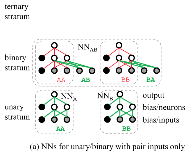
Schematic representation of stratified training of multilayer NNs. Here we show only one hidden layer of neurons and only pair input symmetry functions. Weights and element species shown in bold green are adjusted while the ones in thin red are kept fixed during the training from the bottom up. The letters denote species types in the input vector; for example, AAB describes a triplet symmetry function centered on an A-type atom with A-type and B-type neighbors (the order of neighbors is irrelevant)
Generalized stratified training
In order to extend the stratified procedure to materials with more complex interactions and an arbitrary number of elements, we have considered more flexible NN architectures that still preserve the intact description of the subsystems. Compared to the original stratified NN layout [1], it involves addition of new neurons, shown as green units in below figure, with different connection patterns and conditions.
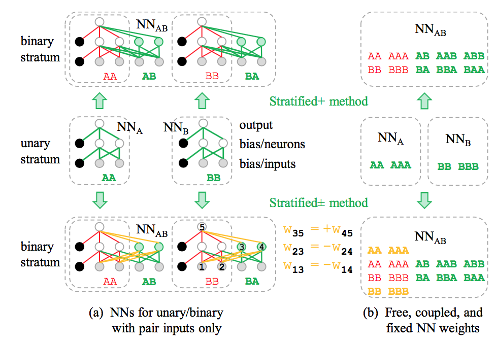
Schematic illustration of stratified+ (top row) and stratified± (bottom row) NN architectures for a binary chemical system. The expansion of the original stratified architecture is done with the addition of new neurons shown in green. The weights of elemental NNs (middle row) are copied and kept fixed in all stratified variations. Free, coupled, and fixed weights are shown in green, yellow, and red, respectively. (a) Connections in a simplified NN with one hidden layer and only pair inputs. The partial constraints shown in yellow and explained in the main text ensure intact description of the elemental structures. (b) Color-coded degrees of weight constraints in NNs with pair and triplet inputs. The original and stratified+ schemes have 60% adjustable weights in the first layer in binaries, 11% in ternaries (e.g., only the last one among AA, AB, AC, AAA, AAB, AAC, ABB, ACC, ABC, see Ref. [1]), and none in quaternaries. The stratified± architecture can be used for an arbitrary number of chemical elements.
The schematic of a ’stratified+’ binary NN (top row in above figure) illustrates that as long as there are no connections from the inputs or neurons in the elemental subnets to the inserted neurons, the new adjustable weights do not alter the signal processing for pure elemental structures. Despite the added flexibility, the NN still does not allow the proper fitting of interactions in compounds with more than three chemical elements. Indeed, the adjustable parts of such NNs involve 60% of inputs in binaries (top right box in above figure), 11% of inputs in ternaries (caption of the above figure) and none for systems with more elements. This restriction is actually imposed by the NN architecture, and can be lifted as follows.
The ’stratified±’ expansion (bottom row in the above figure) introduces semi-adjustable links even in the inherited parts of the merged NN. We add neurons in pairs, coupling the two weights incoming from each subsystem input to have opposite values while coupling the two outgoing weights to be the same. For a purely elemental structure, the interspecies input values are zero and the net signal (at neuron 5) from each elemental input (1) passed through the paired neurons (3&4) will be zero as well regardless of the coupled weight magnitudes. For a binary structure, the non-zero binary inputs multiplied by fully unconstrained weights will unbalance the elemental signals because of the non-linear nature of the activation function resulting in a non-zero contribution at neuron 5 that depends on both elemental and binary (semi)adjustable weights.
The set of new partially constrained weights shown in yellow in the above figure enables the stratified± NN to better capture the screening and charge transfer effects as well as describe interactions in systems with an unlimited number of species. In a trial implementation, we imposed the constraint by penalizing the mismatch between the coupled weights as \(\Sigma_N \sigma(w_{1,N}\pm w_{2,N})^2\). We have observed no need to adjust the \(\sigma\) penalty factor during the NN optimization, as the differences between coupled weight magnitudes become negligible after a few dozen training steps; near the end of optimization, we set the magnitudes to their average and keep them fixed without any appreciable effect on the error. To the best of our knowledge, this semi-constrained solution for systematically expanding NN features has not been considered in the field of materials modeling.
One way to determine whether the use of the expanded NN architectures is warranted is to reoptimize the standard stratified NN without any constraints on the full dataset. A significant reduction in the training and testing errors would indicate the need for additional NN flexibility. In our studies of metal alloys, the error reductions are usually in the 0-15% range (e.g., see Figure 4 in Ref. [1]). Our preliminary tests have shown that both stratified+ and ± architectures end up with errors about midway between those in the stratified and full NNs. In order to quantify the improvements arising from the additional degrees of freedom in each scheme, we plan to investigate more challenging systems comprised of different element types in future studies.