Evolutionary search

Overview

The key features and performance of the evolutionary search (EVOS) are described in Section 6 of Ref. [1]. The evolutionary algorithm (EA) enables an efficient identification of ground state configurations at a given chemical composition. The EA is particularly advantageous in dealing with large structures when no experimental structural input is available [2] [3].

The searches can be performed for 3D crystals, 2D films, and 0D clusters. Population of structures can be generated either randomly or using available structural information. Essential evolutionary operations are ‘crossover’, when a new configuration is created based on two parent structures in the previous generation, and ‘mutation’, when a parent structure is randomly distorted.

For 0D nanoparticles, we have introduced a multitribe EA that allows an efficient simultaneous optimization of clusters in a specified size range [4]. A separate bash script is needed to submit the co-evolutionary search and exchange seeds among tribes at the end of each cycle of isolated evolution.

The EA engine in MAISE expects local relaxations of structures to be performed by an external code (flag CODE) using a queueing system (flag QUET). The current version is linked with VASP for DFT calculations and with MAISE for neural network calculations. The majority of the algorithm’s numerous parameters related to the generation, evolution, and selection of structures have been tuned for typical crystalline unit cells with up to about 50 atoms and clusters with a few hundred atoms.

In order to run an EA optimization, the user should

• configure the setup file (Internal settings)

• place submission files in the INI directory (External settings)

• run maise in the automated or manual mode (Job execution)

Internal settings

All internal settings are specified in the setup file.

Table 1 lists the group of general FLAGs that define the system type, population size, queue type, analysis, etc.

Table 1: General evolutionary search FLAGs.

FLAG	Short description
JOBT	EVOS: auto run (10); soft exit (11); hard exit (12) analysis (13); manual run (14)
NMAX	maximum number of atoms
MMAX	maximum number of neighbors within cutoff radius
NSPC	number of species types
TSPC	species types
ASPC	atom number of each species
CODE	MAISE-INT (0); VASP-EXT (1); MAISE-EXT (2)
QUET	queue type: torque (0); slurm (1)
NDIM	structure type: crystal (3); film (2); cluster (0)
LBOX	box size for clusters or films
NPOP	population size
SITR	starting iteration
NITR	number of iterations
TINI	starting options if SITR=0
TIME	max time per relaxation
PGPA	pressure in GPa
KMSH	reciprocal spacing for VASP KPOINTS generation
DENE	energy window for selecting distinct structures
SCUT	RDF difference for selecting distinct structures
SEED	random number generator seed (0 for system time)

The second group of FLAGs in Table 2 define operations to generate or evolve structures. Structure type in the table below defines the unit cell dimensionality, i.e., 3D for crystals, 2D for films, and 0D for clusters. Zero-parent structures are generated from scratch. One-parent structures are created by modifying a randomly picked structure from a previous generation. Two-parent structures are created by crossover of two randomly picked structures from the previous generation. For crystals and films, creation of initial unit cells is controlled only by TINI while creation of offspring can be done with either MUTE or MATE.

The parameters are fractions from 0 to 1 defining what part of the population will be created with a particular operation. The total must add up to 1. Let’s say the population consists of 20 clusters (NPOP), TETR =0.1, PLNT =0.1, MATE =0.7, and MUTE =0.1. Then the initial population will have 10 TETRIS-type and 10 seeded structures [20*0.1/(0.1+0.1) each]. All other populations will have 2 TETRIS-type, 2 seeded, 14 crossed-over, and 2 mutated clusters.

Table 2: FLAGs defining structure generation and evolution.

FLAG	Operation type	Parent number	Structure type
MATE	crossover with planar cut	2	0D 2D 3D
MUTE	mutation via distortion	1	0D 2D 3D
TETR	generation with TETRIS	0	0D 3D
PLNT	generation with seeds	0	0D
PACK	generation of packed shapes	0	0D
RAND	generation of random shapes	0	0D 3D
SWAP	crossover with sphere cut	2	0D
RUBE	Rubik’s cube mutation	1	0D
REFL	symmetrization via reflection	1	0D
INVS	symmetrization via inversion	1	0D
CHOP	mutation via facet chop	1	0D

The remaining FLAGs in Table 3 specify the mutation and crossover operations.

Table 3: FLAGs defining mutation and crossover operations.

FLAG	Short description	Structure type
ELPS	cluster ellipticity	0D
MCRS	mutation rate in crossover	0D 2D 3D
SCRS	swapping rate in crossover	0D 2D 3D
LCRS	lattice vector distortion in crossover	2D 3D
ACRS	atomic position distortion in crossover	0D 2D 3D
SDST	swapping rate in mutation	0D 2D 3D
LDST	lattice vector distortion in mutation	2D 3D
ADST	atomic position distortion in mutation	0D 2D 3D
MAGN	max number of tries for crossover	0D 2D 3D

JOBT controls the job type and can be changed during the run to stop the evolutionary search run in the automated mode.

• 10 The evolutionary search will auto run from iteration SITR until iteration NITR.

• 11 The auto run will exit at the end of the current iteration.

• 12 The auto run will be stopped, submitted jobs cancelled, and the current iteration deleted.

• 13 Search analysis will examine all created minima stored in the EVOS directory and will select structures within DENE different by at least SCUT.

• 14 The evolutionary run will run manually one generation at a time.

NMAX should be the sum of atoms of all species.

MMAX is the maximum number of nearest neighbors within the 6.0 A cutoff.

NSPC is the number of species, e.g., 2 for a binary compound.

TSPC specifies the atomic number of each species, e.g., ‘5 26’ for B and Fe. In case a neural network model is used, the atomic numbers must be ordered from smallest to largest.

ASPC specifies the number of atoms of each species each unit cell in the population will have, e.g., ‘8 2’ for Fe₂B₈.

CODE specifies what external code will be used for performing local optimizations of structures.

• 1 VASP: calculation at the DFT level

• 2 MAISE: calculation at the neural network level

QUET sets the type of the queueing system for submission of local optimization jobs with the external code specified by CODE.

NDIM is the dimensionality of the system. 3D crystals are fully periodic. 2D films are periodic in (x,y) and constrained to the (x,y) plane, with the c lattice vector specified by LBOX. 0D clusters are non-periodic, with all 3 lattice vectors set to LBOX.

LBOX is the fixed lattice vector length in A for simulating 2D films or 0D clusters. The a and b lattice vectors in films can be arbitrary. In DFT calculations, the LBOX value should be just large enough, e.g., 18-20 A for clusters with 50-100 atoms, to ensure at least 8-10 A between atoms in different unit cells along non-periodic directions. In NN calculations, LBOX should ensure at least R_c separation between atoms in different unit cells; it can be arbitrarily large because, in contrast to the case of DFT, it does not affect the calculation speed. R_c is the interatomic interaction cut-off parameter specified for a NN potential at the end of the model file.

NPOP specifies the number of structure members in the population. It is good practice to set the value to at least the total number of atoms in the unit cell, e.g., 16-32 for 16-atom structures. The code will generate NPOP offspring members and submit them to the queue separately in each generation.

SITR specifies the starting iteration. For a new evolutionary run, set it to 0. For continuing a finished run, set it to the previous NITR value; in this case, MAISE will read in the population from the EVOS/GXXX directory, where XXX is (NITR-1).

NITR is the total number of generations which can be changed during the evolutionary run. As the global search convergence is highly dependent on the species types and the system size, there is no single value that can ensure the location of the ground state. Searches for 3D crystals with up to 10 atoms typically converge within 100-500 local optimizations defined as NPOP × NITR. Larger 3D systems with 16-28 atoms per unit cell can take 1000-5000 local optimizations.

TINI specifies how structures will be generated in a new search (if SITR is not 0 the code will ignore the TINI option and simply use the last generation).

• 0 Structures will be generated randomly.

• 1 The code will use INI/POSCAR000 and randomize the atomic positions and lattice vectors. This option dramatically accelerates finding (meta)stable configurations related to the specified structure.

• 2 The code will use the lattice vectors from INI/POSCAR000 and generate atomic positions randomly. This option is helpful, e.g., when the lattice constants are known from experiment.

• 3 (Beta version) The code will use the lattice vectors from INI/POSCAR000 and space group from INI/SYMINI000 to generate unit cells with the specified symmetry. The operation will choose random Wyckoff positions and generate random values for non-fixed Wyckoff parameters. The space group must be specified in the following format:

115
8 l  x    y    z  	
4 k  x   0.5   z  	
4 j  x   0.0   z  	
4 i  x    x   0.5  	
4 h  x    x   0.0 	
2 g 0.0  0.5   z  	
2 f 0.5  0.5   z  	
2 e 0.0  0.0   z  	
1 d 0.0  0.0  0.5 
1 c 0.5  0.5  0.5 
1 b 0.5  0.5  0.0
1 a 0.0  0.0  0.0

TIME specifies the maximum time in seconds allowed for a local structure relaxation with an external code. The time starts after a job starts running. Once the run time exceeds the specified value, e.g., in case the relaxation is stuck or the node is down, the code will delete the job. A message of the failed relaxation will be written to log.out. In case too many relaxations fail in the zeroth generation, the search will be terminated. A typical VASP relaxation job in evolutionary runs for medium-size structures with 8-12 atoms is under 9600 seconds on 16 cores. A typical MAISE job for up to 100-atom structures is under 600 seconds on 16 cores.

PGPA sets a target hydrostatic pressure. The value will be used to update INI/INCAR0 for VASP jobs and INI/NNET/setup for MAISE jobs.

KMSH defines the reciprocal spacing in 1/A to generate KPOINTS for VASP calculations. If the relaxation involves several cycles with different levels of accuracy it is better to use a separate script to generate a k-mesh with the desired cycle-dependent density. A custom Python script is available upon request.

DENE is an enthalpy window in eV/atom for selecting relevant structures during a Search analysis job. 3D systems typically have a few different local minima within 0.010-0.020 eV/atom above the most stable structure.

SCUT is the RDF difference for finding distinct structures during a Search analysis job. The selection proceeds from the most stable structure up the enthalpy-ranked list. If SCUT is set, e.g., to 0.95, a structure that has a scalar product with an already selected structure above this SCUT value will be considered too similar and not included.

SEED specifies the starting seed of the random number generator. It should be set to zero to generate the seed from the system time and define a unique run.

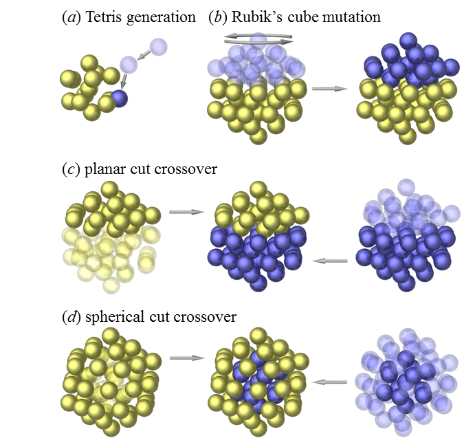
Illustration of select generation and evolution operations for clusters.

MUTE defines what fraction of the population that will be generated with a mutation operation. For arandomly picked parent structure, it will displace the atomic positions by a distance specified by ADST, distort the lattice constants by a fraction specified by LDST, and perform swaps of atomic positions defined by SDST.

MATE defines what fraction of the population that will be generated with the crossover operation using two random parents from a previous generation. Two parent structures are sliced approximately in half with a planar cut.

TETR defines what fraction of the population of 0D clusters or 3D crystals that will be generated randomly at the beginning or during the run using the TETRIS operation introduced in our recent study [4]. For clusters, it involves shooting atoms one by one toward the origin from different random directions and keeping each atomic position closest to the origin. For crystals, it involves a similar approach but atoms are dropped down along the c axis.

PLNT defines what fraction of the population of 0D clusters that will be ‘planted’ at the beginning of an evolutionary run by randomly picking one of the seed structures provided by the user as INI/POSCARXXX where XXX ranges from 0 up to NPOP. As described in [4], a few atoms on these clusters’ surface will be adjusted to explore close surface configurations. In case of multitribe co-evolution, the seed clusters can have different number of atoms, as the code will either remove atoms randomly from the surface or add atoms randomly to the surface to achieve the target number. This option currently works only for a single species.

PACK defines what fraction of the population of 0D clusters that will be generated at the beginning of an evolutionary run by creating ordered structures with FCC, BCC, or HCP lattice with random facets. The type of the 3 lattices is chosen randomly.

RAND defines what fraction of the population of 0D clusters or 3D crystals that will be generated randomly at the beginning or during the run using the RAND (formerly BLOB) operation operation [4]. For clusters, atoms are placed randomly within a sphere with an estimated cluster radius and then readjusted with a repulsive potential to ensure physical distances. The sphere can be made into an ellipsoid with an ELPS parameter to promote construction of non-spherical shapes.

SWAP defines what fraction of the population of 0D clusters that will be generated with the crossover operation using two random parents from a previous generation. Two parent structures are sliced with a spherical cut, i.e., the offspring inherits the core from one parent and the shell from the other. The operation was introduced for testing purposes and turned out to be less efficient than the standard crossover operation MATE with the planar cut [4].

RUBE defines what fraction of the population of 0D clusters that will be generated with a Rubik’s cube operation. The transformation involves a rotation of approximately half of a parent structure along a randomly chosen axis by a random angle. The operation proved to be comparable in efficiency to the standard crossover MATE [4].

REFL defines what fraction of the population of 0D clusters that will be generated with a reflection operation. A parent structure is sliced with a planar cut approximately in half and only one half is kept. The missing half is regenerated by applying mirror symmetry across the plane used for the cut. Any pairs of atoms of the same species that happen to be too close to each other are merged into one.

INVS defines what fraction of the population of 0D clusters that will be generated with an inversion operation with the same idea as the reflection operation REFL.

CHOP defines what fraction of the population of 0D clusters that will be generated with a chop operation that helps create facets. Up to square root of the total number of atoms are selected with a single planar cut and relocated to random positions on the opposite side.

ELPS is a dimensionless parameter defining the ellipticity of the cluster shapes generated with TETR and RAND operations. It is introduced to promote the introduction of non-spherical motifs in the population. A value of 0.3 will tell the code to pick the ellipticity parameter randomly between 0.7 and 1.3. The principal axis will be randomly oriented along x, y, or z.

MCRS defines the mutation rate in crossover operations. Note that this additional mutation is applied after the structure is created with the crossover.

SCRS defines the swapping rate in crossover operations if the structure is selected to have an additional mutation. It means that for systems with more than one species type, the code will perform MCRS × NMAX swaps of atomic positions.

LCRS defines the lattice vector distortions in crossover operations if the structure is selected to have an additional mutation. A typical 0.1 dimensionless value means that the lattice vector components will be distributed primarily between 0.9 and 1.1 of the original values according to the normal distribution. It must be set to zero for clusters.

ACRS defines the atomic position displacements in crossover operations if the structure is selected to have an additional mutation. A typical 0.1 A value means that atoms will be displaced by a random distance primarily within the 0.1-A sphere from the original position.

SDST defines the swapping rate in mutation operations. It means that for systems with more than one species type, the code will perfom MCRS × NMAX swaps of atomic positions.

LDST defines the lattice vector distortions in mutation operations. A typical 0.2 dimensionless value means that the lattice vector components will be distributed primarily between 0.8 and 1.2 of the original values according to the normal distribution. It must be set to zero for clusters.

ADST defines the atomic position displacements in mutation operations. A typical 0.2 A value means that atoms will be displaced by a random distance primarily within the 0.2-A sphere from the original position.

MAGN is the maximum number of tries per generation allowed to create the set of new structures in the crossover operations. For populations with very different motifs, e.g., with large mismatches in crystal unit cells or cluster shapes, it may be difficult to find two compatible parent structures that will produce an offspring with physically meaningful distances. The code will exit if the number of attempts exceeds the default 1000000 value. Setting MAGN to 10000000 is recommended for larger structures.

External settings

Please place the following input and submission files into the INI directory.

VASP calculations

• sub0 is a submission file that defines the queue type, the number of cores/nodes, the number of relaxation steps, etc.

#!/bin/bash
#SBATCH -p long
#SBATCH -n 16
#SBATCH -N 1

cd $SLURM_SUBMIT_DIR
EXE=vasp
MPIRUN=mpirun

cd EVOS/GGGG/MMMM/

date -d now +%s > stamp

# ============= relaxation 1 =============
sed -i 's/NSW=0/NSW=11/' INCAR
mpirun $EXE  > out

mv POSCAR    POSCAR.1
mv CONTCAR   CONTCAR.1
mv OUTCAR    OUTCAR.1
mv OSZICAR   OSZICAR.1

# ============= relaxation 2 =============
cp CONTCAR.1 POSCAR
sed -i 's/norm/acc/' INCAR
sed -i 's/NSW=11/NSW=21/' INCAR
mpirun $EXE  > out

mv POSCAR    POSCAR.2
mv CONTCAR   CONTCAR.2
mv OUTCAR    OUTCAR.2
mv OSZICAR   OSZICAR.2

# ============= static run   =============
cp CONTCAR.2 POSCAR
sed -i 's/NSW=21/NSW=0/' INCAR
mpirun $EXE  > out

mv POSCAR    POSCAR.0
mv CONTCAR   CONTCAR.0
mv OUTCAR    OUTCAR.0
mv OSZICAR   OSZICAR.0
# ========================================
 
rm IB* EI* PC* XD* CH* WA* vasp* DO* 
cd ../../..

• POTCAR defines the pseudopotential in VASP calculations. Make sure that the species order is consistent with TSPC !

• INCAR0 sets up VASP calculations.

• KPOINTS is optional. There are three ways to specify k-mesh:

  • define KPOINTS file for each relaxation cycle in INI and copy it to the work direcory; to be used in searches with fixed unit cells

  • define KMSH in setup that will generate a single KPOINTS with targeted spacing in the reciprocal space

  • use a custom python script to generate KPOINTS for each cycle; available upon request

• POSCAR000 is optional for seeding the search, see TINI and PLNT.

It is advisable to run a few cycles of local optimizations and finish the calculation with the most accurate ‘static’ run. Note that MAISE will only read the final enthalpy from OUTCAR.0.

MAISE calculations

• sub0 is a submission file that defines the queue type, the number of cores/nodes, the number of relaxation steps, etc.

#!/bin/bash
#SBATCH -p tera
#SBATCH -n 1

cd $SLURM_SUBMIT_DIR

cd EVOS/GGGG/MMMM/

date -d now +%s > stamp

cp -r ../../../INI/NNET/* .

maise-nnet > out

mv POSCAR    POSCAR.0
mv CONTCAR   CONTCAR.0
mv OUTCAR    OUTCAR.0
mv OSZICAR   OSZICAR.0

rm -rf setup tmp* wyck* mod* maise-nnet
cd ../../..

• NNET/setup sets up MAISE local relaxation jobs. Make sure to check

  • NPAR parallelization parameter

  • MITR iteration number

  • PGPA external pressure

• NNET/model defines the interatomic potential for the MAISE local relaxation job.

• NNET/maise-nnet is the standard MAISE executable that will perform the local relaxation.

• POSCAR000 is optional for seeding the search, see TINI and PLNT.

Job execution

An evolutionary search can be run either in automated (JOBT = 10) or manual (JOBT = 14) mode as described below.

Search auto run

The automated evolutionary optimization (JOBT = 10) is launched by running MAISE in the background as

$ nohup maise &

The search (re)starts from a given generation and proceeds for a specified number of iterations (FLAG NITR). In each cycle, the code generates a new population, submits a job for each structure to a specified queue, checks if the jobs finished successfully, processes the results, and outputs enthalpy and volume for each structure.

During the local optimizations performed externally, the evolutionary search job uses virtually no CPU resources and only checks the status of local optimizations every 5 seconds. Since running programs in the background is discouraged on most supercomputers, an evolutionary search can be run alternatively in the manual mode.

Search manual run

The manual evolutionary optimization (JOBT = 14) is done by running MAISE once per generation (the SITR and NITR FLAGs are ignored in this case):

$ maise

Each execution of the code will analyze the previous generation, write down the information to eXXXX.dat files as described in the following section, generate new structures in the EVOS/GXXX/ directory, and create submission scripts gYYY in the working directory for running each structure.

For example, in a search with 10 members per population and two completed generations EVOS/G001/ and EVOS/G001/, the code will create 10 subdirectories EVOS/G002/M010/ through EVOS/G002/M019/ with one new offspring structure in each. The corresponding scripts g010 through g019 can be submitted to compute nodes. If the jobs are run elsewhere, one should replace the M010/-M019/ directories in EVOS/G002/ with the completed runs. The subsequent execution of MAISE will process the results and generate the next set in EVOS/G003/.

Search check

The search engine launched in the automated mode can complete the global optimization without any supervision. However, it is good practice to monitor the progress by checking the following output files. Note that MAISE reads the final enthalpy in external VASP or MAISE runs from OUTCAR.0 in each EVOS/GXXX/MYYY directory.

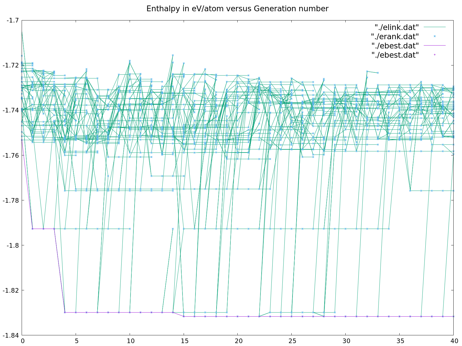
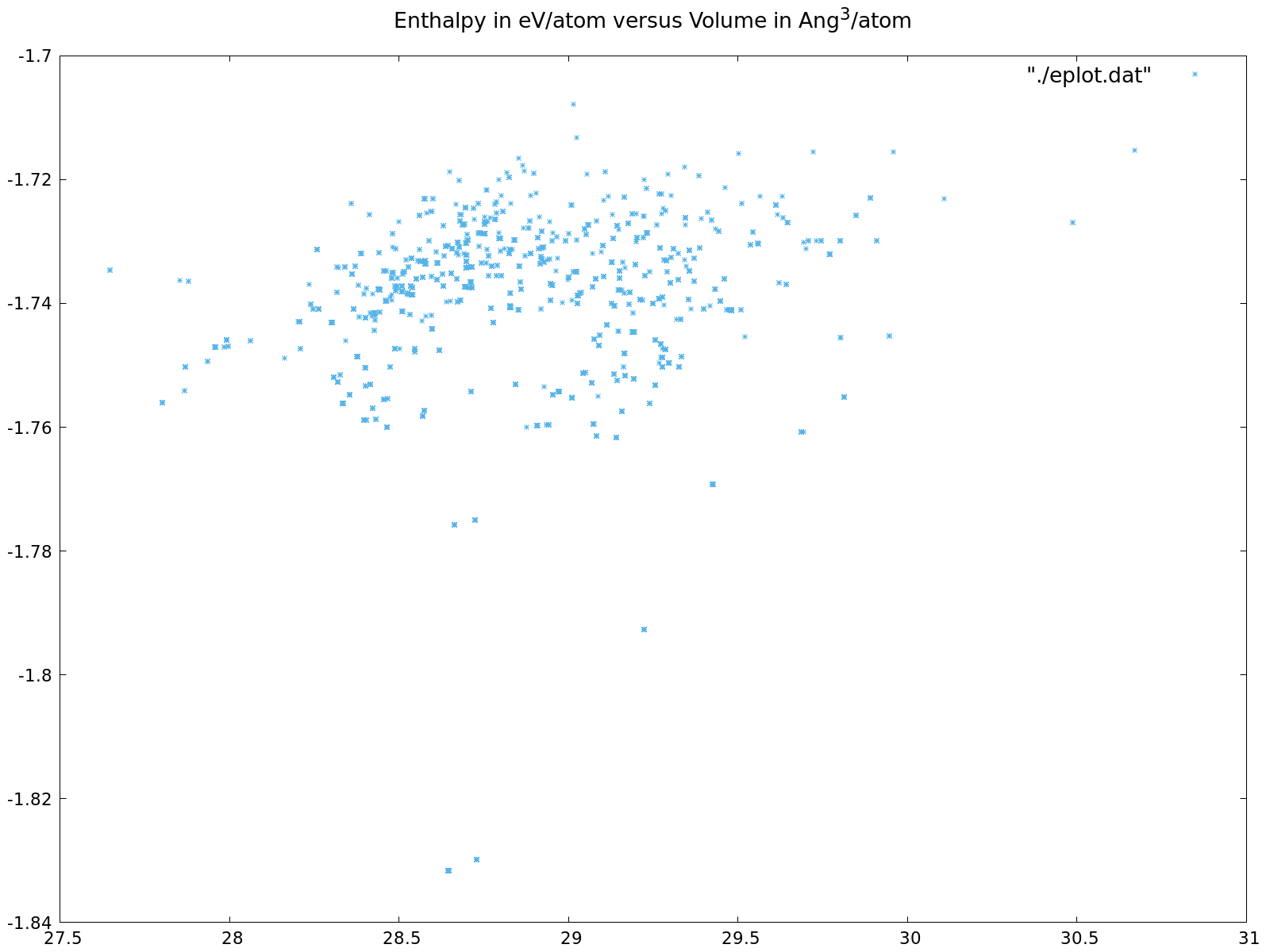
• log.out stores all MAISE messages about structure generation, structure selection, etc.

• EVOS/GXXX/MYYY stores results for YYYth member in the XXXth generation (see note below).

• ebest.dat stores the enthalpy in eV/atom for the best member in each generation.

• erank.dat stores the enthalpy in eV/atom for each member in each generation.

• eplot.dat stores enthalpy vs volume in eV/atom vs \(A^{3}\)/atom for all minima.

• elink.dat stores heredity for each offspring.

Note that each EVOS/GXXX contains double the population size NPOP: directories numbered from NPOP to (2 * NPOP - 1) have optimization runs with offspring, while directories numbered from 0 to (NPOP - 1) have the new population chosen from the pool of old parents and new offspring.

By running the following bash script plot during or after the evolutionary run, one can visualize the information in these files.

$ plot

#!/bin/bash
dir=.
file=eplot

gnuplot -persist <<-EOF

set terminal pngcairo size 1600, 1200
set output 'collection.png'
set title 'Enthalpy in eV/atom versus Volume in Ang^3/atom'
set tics  font ", 16"
set key   font ", 20"
set title font ", 20"
set autoscale
plot  "$dir/$file.dat" with points ls 3

EOF

dir=.
file1=elink
file2=erank
file3=ebest

gnuplot -persist <<-EOF

set terminal pngcairo size 1600, 1200
set output 'evolution.png'
set title 'Enthalpy in eV/atom versus Generation number'
set tics  font ", 16"
set key   font ", 20"
set title font ", 20"
set autoscale
plot  "$dir/$file1.dat" with line   ls 2, \
      "$dir/$file2.dat" with points ls 3, \
      "$dir/$file3.dat" with line   ls 1, \
      "$dir/$file3.dat" with points ls 1

EOF

The energy profile and structure heredity are shown in evolution.png.

The distribution of enthalpy vs volume is shown in collection.png.

Search analysis

After a search is completed, one can perform a separate analysis job to select most relevant distinct local minima. Please set JOBT to 13, adjust DENE and SCUT, and run MAISE:

$ maise

The analysis output with DENE = 0.040 eV/atom and SCUT = 0.99 for an evolutionary search for Mg₈Ca₄ modeled with a neural network potential is shown below.

   0  28.645994 -1.831614   0 
   1  28.728507 -1.829820   0 
   2  29.223607 -1.792665   0 
   0 194 hP12
   1 227 cF24
   2  12 mS24
Found   6400 candidates with lowest enthalpy -1.831614
Found    304 structures with enthalpy range  -1.831614 -1.791614
Found      3 structures with enthalpy range  -1.831614 -1.791614 different by CxC  0.990000

In this case, MAISE scanned all 6400 structures stored in EVOS, found 304 of them to be within the specified 40 meV/atom window, determined that only 3 of them were unique based on the specified 0.99 scalar product cutoff, and found space groups along with Pearson symbols for the structures in the selected group. The corresponding original POSCAR files were placed in the POOL and POOL/SET0 directories.

Note that at least half of the saved 6400 structures appear twice because EVOS keeps both parent and offspring structures in each generation. In addition, some minima may be found independently multiple times during the search. For this reason, the 304 found minima within 40 meV/atom are likely true duplicates rather than closely related structures. The existence of only 3 unique structures in such a large enthalpy window is unusual. Typically, one finds dozens of crystal structures within 10 meV/atom and hundreds of cluster structures within 5 meV/atom.

Additional analysis can be performed by running several consecutive JOBT = 13 runs as described below. It is intended primarily for checking and comparing the results of NN-based searches with DFT.

The first pass will collect all finished runs in EVOS, save select structures in POOL/SET0, and write the analysis results in ana0.dat. Make sure that the pool size is not too large by checking ana0.dat, adjusting the DENE and SCUT selection criteria, and re-running the analysis as needed. In case the code finds that``POOL/INI0`` directory is present, it will submit further relaxation and symmetrization jobs for each structure in POOL/SET0` using NN settings in ``POOL/INI0 and outputting the results in POOL/RUN0. Make sure all the jobs are finished before proceeding with the next analysis step.

The second pass will automatically detect all finished runs in POOL/RUN0, save select structures in POOL/SET1, and write analysis results in ana1.dat. Now, if POOL/INI1 is present, the run will additionally submit relaxation jobs for each structure in POOL/SET1` using DFT settings in ``POOL/INI1 and outputting the results in POOL/RUN1. Again, it is a good idea to check the pool size and adjust the DENE and SCUT settings before placing INI1 into POOL. Make sure all the jobs are finished before proceeding with the next analysis step.

The final pass will automatically detect all finished runs in POOL/RUN1, save select structures in POOL/SET2, and write analysis results in ana2.dat.

The post-search finer relaxation of a small pool of structures allows one to use shorter relaxation during the searches. Note that EVOS is analyzed when neither POOL/RUN0 nor POOL/RUN1 is present, while POOL/RUN0 is analyzed when POOL/RUN1 is not present.

Search example

An example available on Github sets up an evolutionary search for Mg₈Ca₄ using our neural network interatomic potential.